
The JAVA version
The JAVA version has compared to the DOS version speeded up the program thousand times, and there is no longer any restrictions on the number of steps in the runs.
Download JAVA standard edition at Oracle: https://www.java.com/en/
Download datasheet for AXIS110J.
The Control Panel
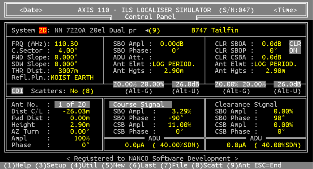
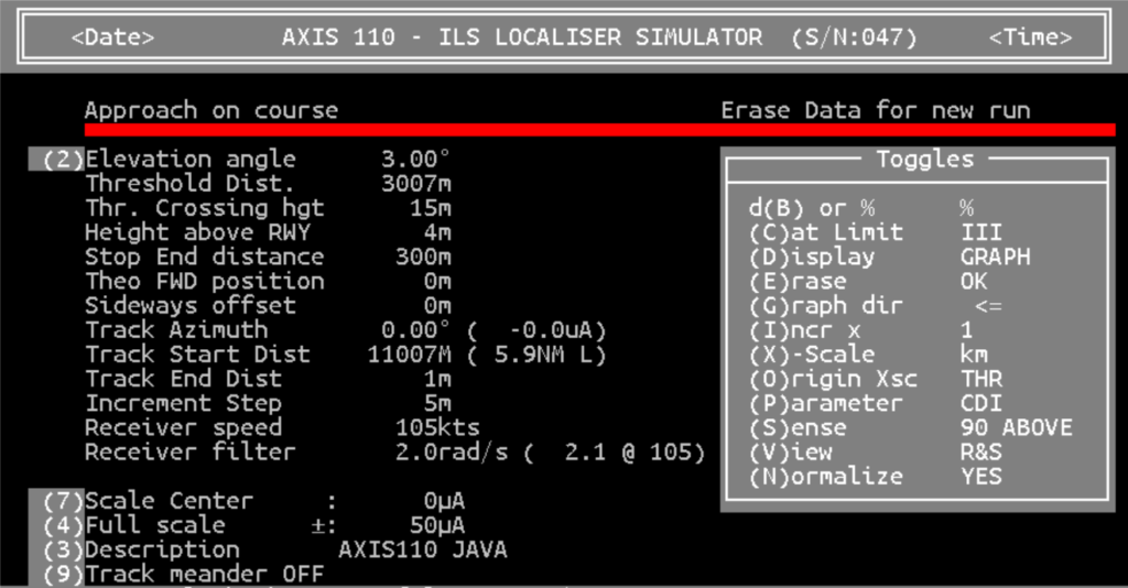
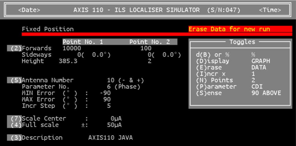
The Control Panel as it appears quite familiar to earlier versions. The (F)-keys are replaced with pure number keys (1), (2)……(9) due to the design og Lap Tops where two keys must be pressed in order to operate a function key. Apart from that the menues and way of using the panel is similar to the DOS version.
The antenna system used in these pages is Normarc 7220 (20 element).
The Menu
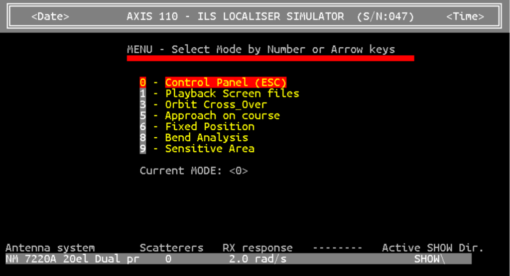
The menu for selecing the five modes available
The Orbit Mode
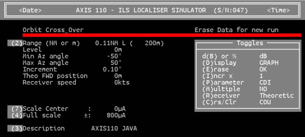
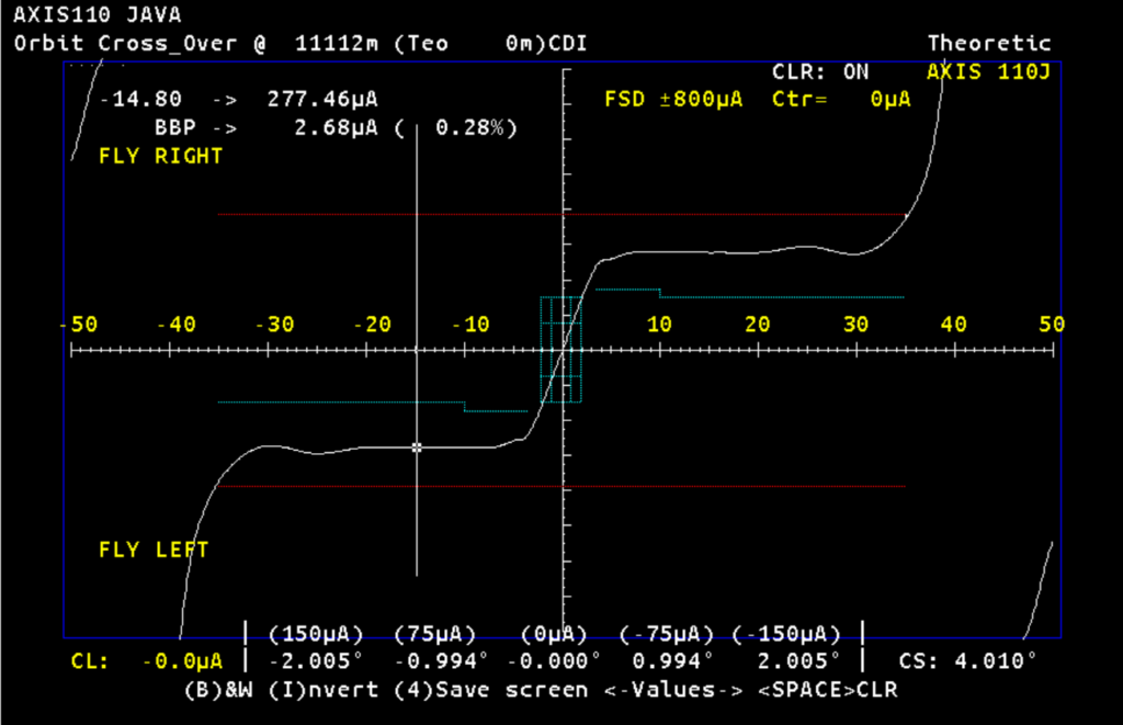
The Orbit mode where the left-right keys are used to check the value along the curve. The values at 14.8°are CDI 277.46uA and BBP 0.28%.
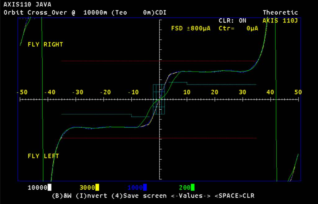
You may run until 6 scans at different distances from the antenna system. Far field at 10,000 meters can be compared to values at closer distances. Here 3000m (yellow), 1000m (blue) and near field at 200m (green).
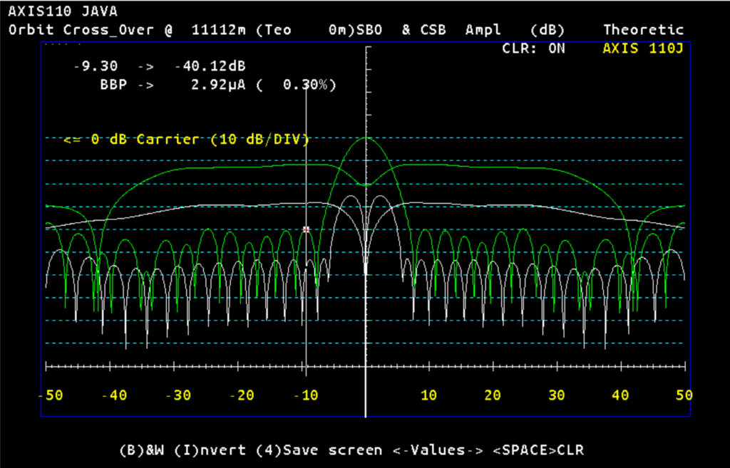
The (P)arameter is changed from (C)DI to (A)mplitude as either percent (%) or d(B). The Course and clearance amplitude, where CSB is green, and SBO white
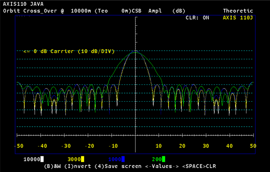
CSB Amplitude at four different distances, 10000m (white), 3000m (yellow), 1000m (blue) and 200m (green).
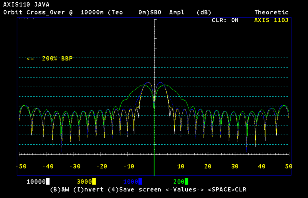
SBO Amplitude at four different distances, 10000m (white), 3000m (yellow), 1000m (blue) and 200m (green).
The Approach Mode
All selections that can be made.
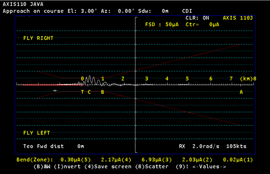
There is a reflection from a hangar, and the disturbances just before the threshold are mainly caused by the clearance signal. This can be proved by switching the clearance off by the Alt-C keys.
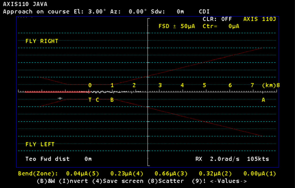
Similar situation as the previous figure, but here the clearance signal is OFF. This check is a smart way to see if the clearance signal has any influence on the complete signal.
The Fixed Position Mode
Two fixed positions at different locations are compared while one of the feed parameters is adjusted within a defined range. Normally the far field is one position, and the other is in the near field, on the runway or at the monitor position.
In the following four figures the two positions are far field (10000m on centreline) and the course line monitor position 100m in front of the antenna system.
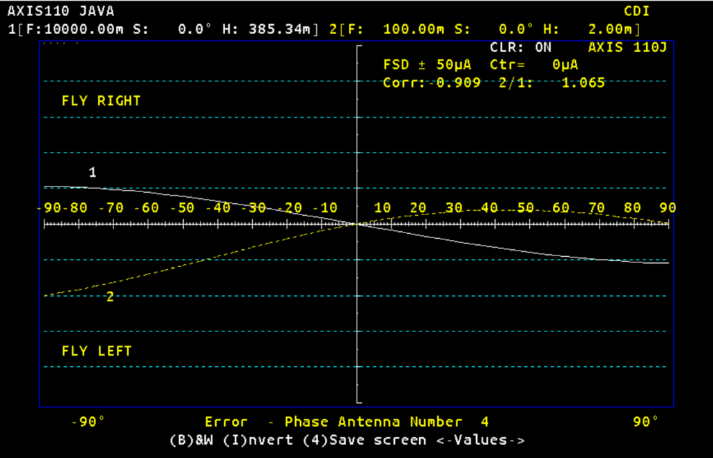
Phase error ±90° in antenna #4. The far field and monitor react in opposite ways
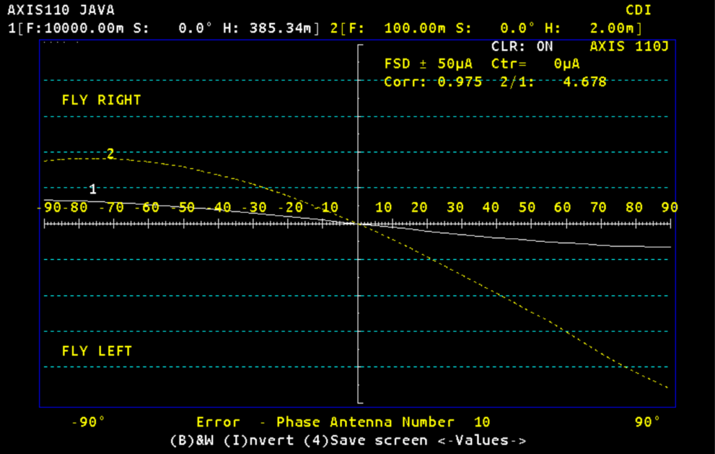
Phase error ±90° in antenna #10. The monitor reacts much more than the far field.
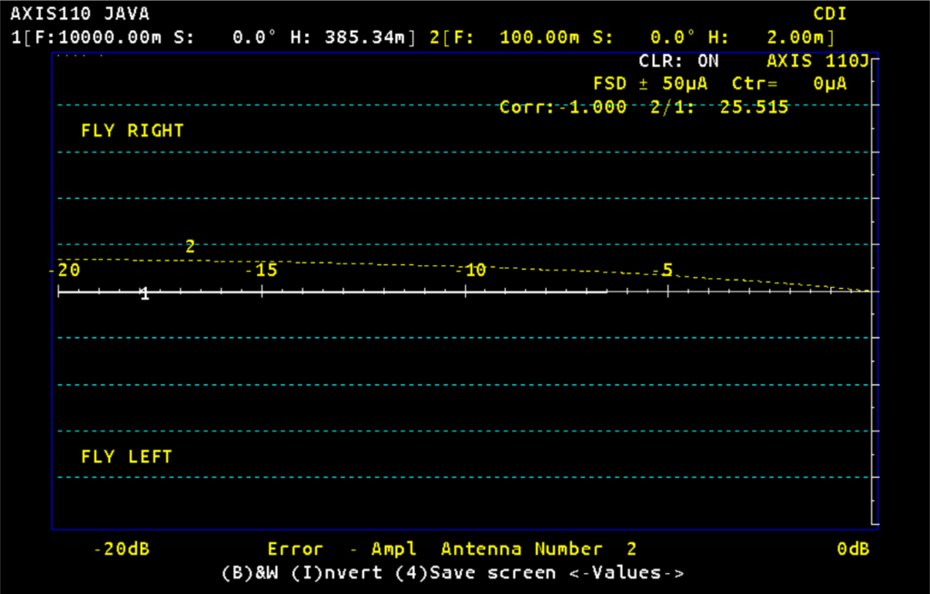
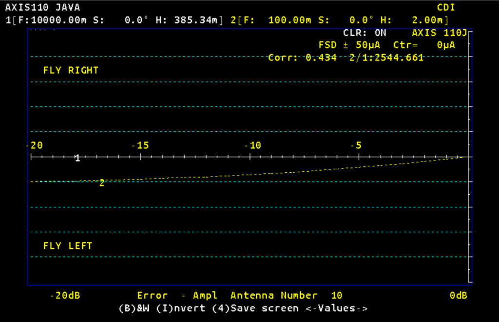
Amplitude error 0 => -20dB in antenna #2. The far field will not react to changes in the amplitude, but the monitor in the near field will. It will get a FLY RIGHT reaction .
Amplitude error 0 => -20dB in antenna #10. The far field will not react to changes in the amplitude, but the monitor in the near field will. It will get a FLY LEFT reaction.
The Bend Analysis Mode
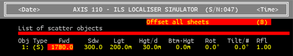
First we put a reflection object in the model. A hangar wall nearly 1800m in front of the localiser, and 300m to the side of the runway centre line. To find the origin of the source of reflection, we need to find the bend length at two different distances. We are starting with finding two half cycle bends (more exact), and convert them to full bend lengths.
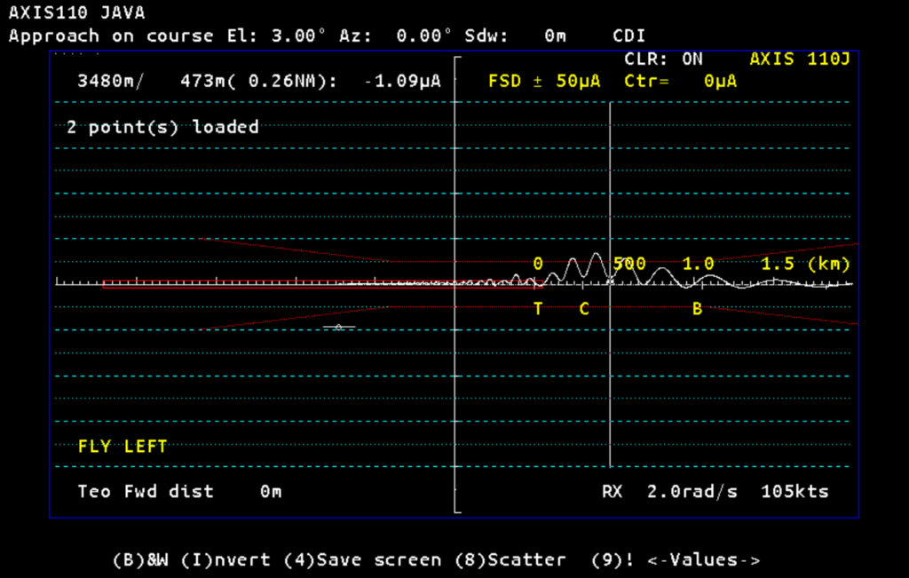
Select a sine wave looking bend, and find the extreme point, either at the top or bottom of a half cycle. Press 0 (zero) to start measuring the bend length.
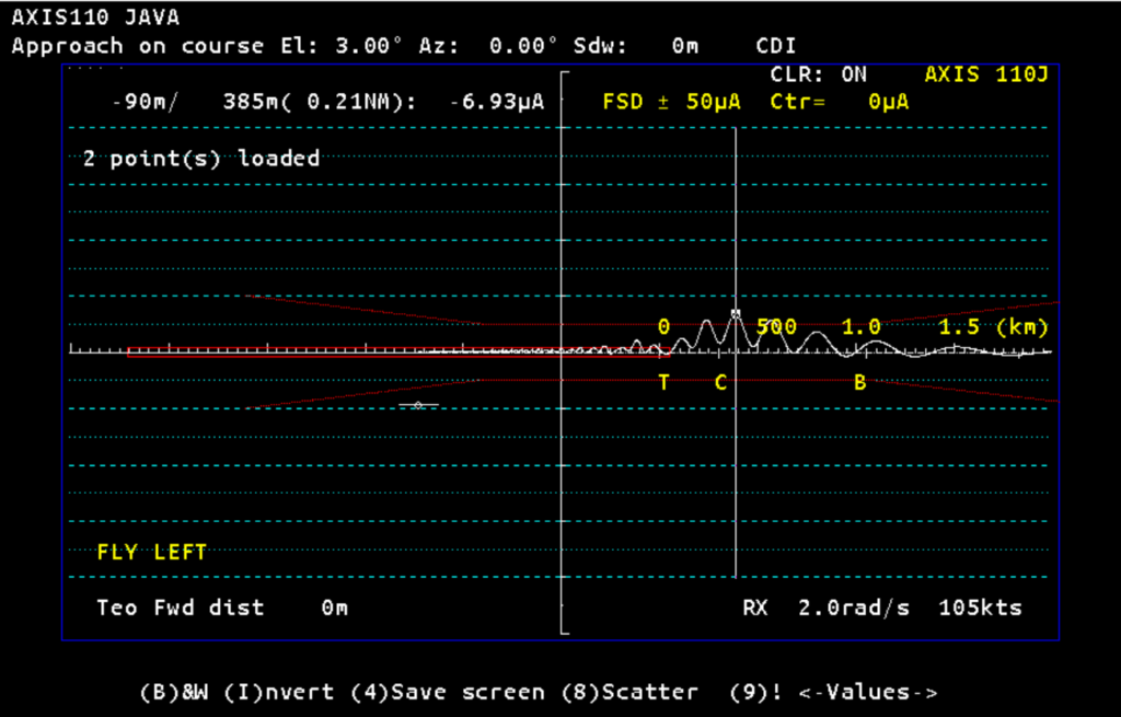
Move the cursor towards the antenna system, and stop at the other extreme. The half bend cycle is 90m, and convert thar to a full length by pressing (2). Meaning you multiply 90m by two and get a bend length at that distance from the antenna system.
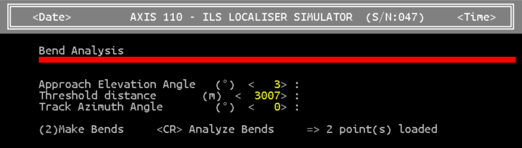
After repeating that somewhere else along the approach, or even select three locations, press <CR> (Enter key) to analyze.
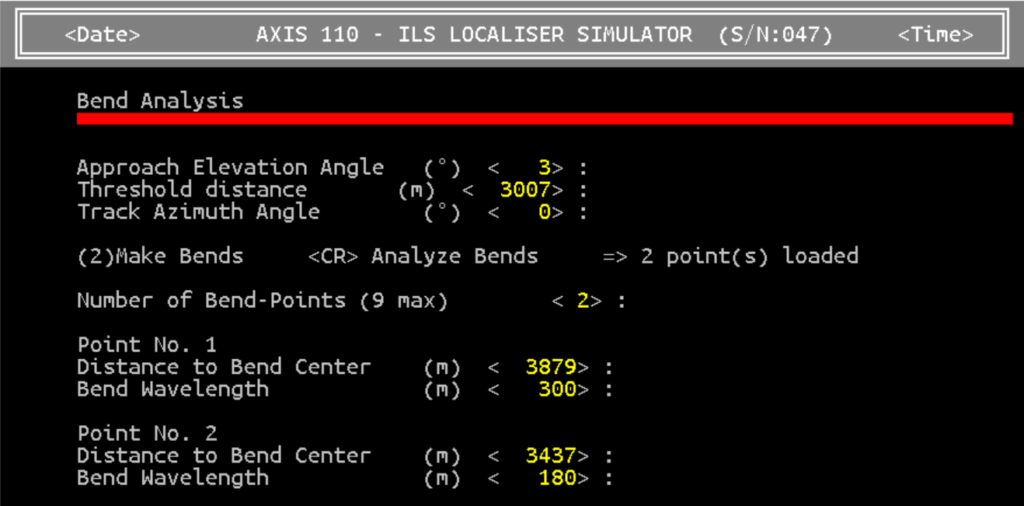
These are the results, showing two different bend lengths at two different distances. The more different the bend lengts are, the better resolution in the final result.
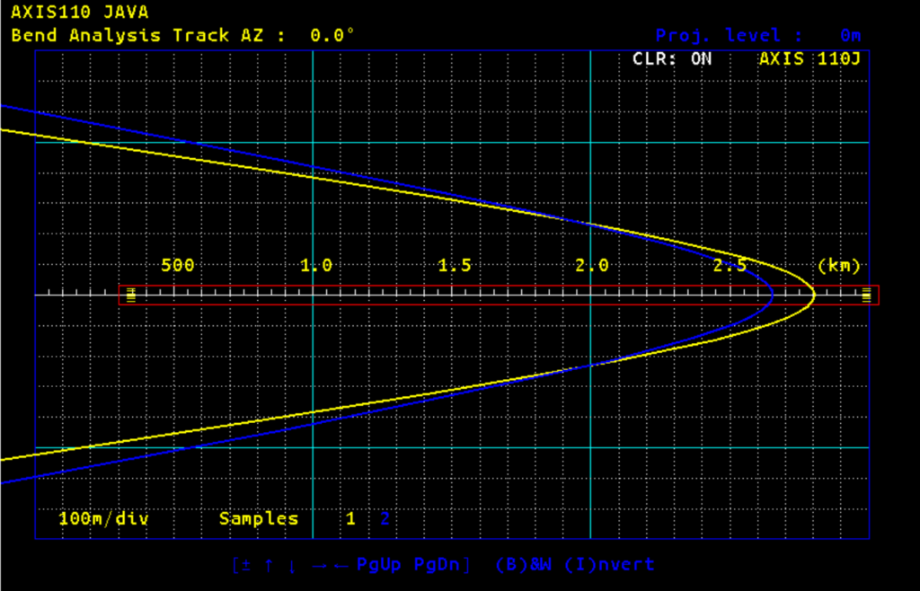
The yellow and blue curves seem to cross near 2.0 km from the antenna system. Use the PgDn key and Arrow right keys to zoom in.
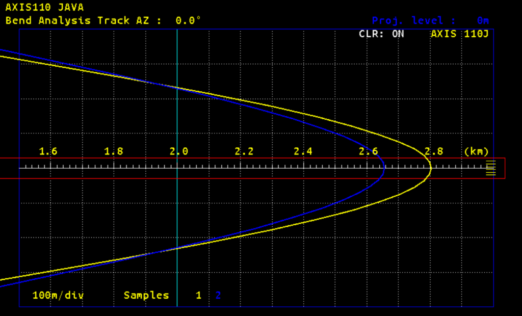
This shows the crossing seems to be at 1850m, and only 250m from the centreline. Not exact, but near enought to find the object if you look around. You will no be in doubt if there is a real hangar there. Note that you get a symmetrical result on each side of the runway, but only one is the real one while the other is an image.
The Sensitive Area Mode
This mode maps the size of the sensitive area for a given situation based on the antenna system chosen in the Control Panel. The sensitive area is where an aircraft on the ground will produce disturbances to the localiser signals received by another aircraft descending along the approach path. The first aircraft will pass through the localiser sector beam when exiting the runway after landing. It is mainly the size and direction (orientation) of the tailfin we are concerned about.
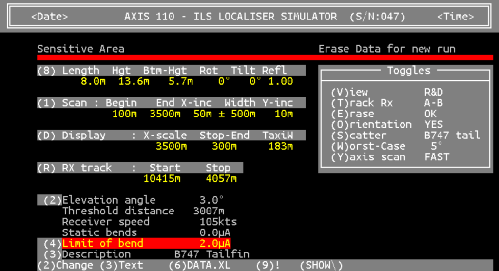
On this page we are setting the most important parameters:
(T) – Track path of the next aircraft, normally ILS point A to B
(O) – Display the worst orientation (direction) of the tailfin
(S) – Select a ready made size of the tailfin, or (8) edit a custom size
(W)– Number of degrees interval to find the worst case orientation
(4) – Choose the limit of maximum bend amplitude disturbance in µA
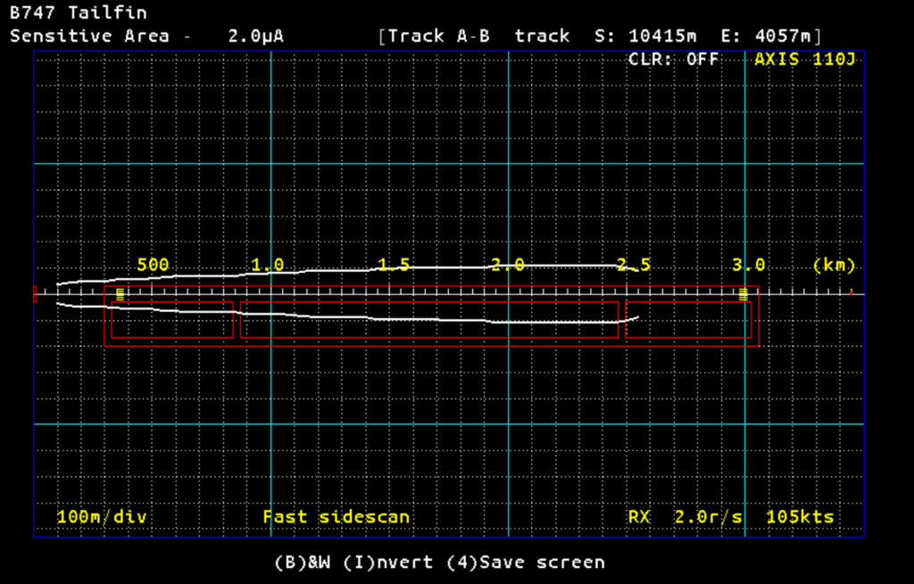
Example showing the size of the sensitive area for a Boeing 747 on exit from the runway after landing. The maximum allowed disturbance is set to 2µA, and each small square is 100m in size. The increment steps for scanning the area is 50m in forward direction and 10m sideways, and these can be edited to any other value using the (1) key.
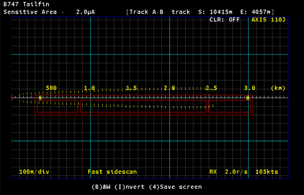
These plots show the worst case orientation of the tailfin, giving the strongest disturbance towards the next approaching aircraft. Due to diffraction of the largest area illuminated from the LOC, the worst angle is often 90° relative to the runway direction.
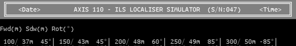
Use the (9) key to display a table of the plots: Distance from the LOC antenna/Distance from RWY CL/Orientation relative to RWY direction.
Training
We will be happy to give you a one week training course covering both AXIS110J and AXIS330J. Under Training you will find either Advanced ILS Course or AXIS User Course at your discretion.
End of AXIS 110 JAVA presentation